Datasets Deep Learning Client App Tutorial

Video Tutorial

The purpose of this sample project is to show you how to use datasets and datascience to predict if a customer loan will be accepted or denied.

The video tutorial below summarizes the steps you need to take to build the deep-learning model using the datasets.
In the next sections you will find the detailed transcript of the video and the code lines.

Two copies of datasets from FusionCreator will be used: Customer Loans and Demographics. The copies are downloaded from your Azure BlobStorage.

Get it from GitHub

If you have a GitHub account, here’s the link to the sample app repository: https://github.com/FusionFabric/ffdc-sample-deeplearning

Clone it and follow the instructions from the README.md file.

Prerequisites

To start building this client application

You must register an application on FusionCreator that includes the two previously mentioned datasets from the Dataset Catalog. After registration, download the datasets from Azure. See step 6 from the Application Wizard and Datasets for more information.
You need a recent Python installation on your machine. However, due to the dependency on the keras library, you must install a compatible Python version, such as 2.7 or 3.6, or previous versions. See the library repository Readme.md for details.
Install Jupyter Notebook, that allows you to run the deep-learning program found in GitHub repository: pip install notebook.
Install the Python libraries that you will use for this sample application:

pip install pandas numpy scipy matplotlib gmaps sklearn keras tensorflow

Create a Python model file and name it datasets-neural-network.py. You will add here all the required code for your client application.
Copy the following code to your model file to import the libraries into your model, in order to handle and manipulate the datasets.

#Data Handling and Manipulation
import pandas as pd
import numpy as np
pd.set_option('display.max_columns', None)  

#Statistical Analysis
from scipy import stats

#Plotting and Visualization
import matplotlib.pyplot as plt
import matplotlib.pylab as plt
plt.rcParams['figure.dpi'] = 120
import gmaps
!jupyter nbextension enable --py gmaps

#Machine Learning
from sklearn.preprocessing import MinMaxScaler
from keras.models import Sequential
from keras.layers import Dense, Dropout
from sklearn.model_selection import cross_val_score, train_test_split
from sklearn.model_selection import KFold
from sklearn.ensemble import RandomForestClassifier

Load Data

In this section you load the Customer Loans and Demographics datasets you downloaded from your Azure Data Share. Create a folder named Data in your working directory. Copy the datasets to this folder.

Load the customer_loans.csv dataset to your model and see its top 5 entries:

df_loans = pd.read_csv('Data/customer_loans.csv',sep=',')
df_loans.head()

Load the customer_demographics.csv dataset to your model and see its top 5 entries:

df_customer = pd.read_csv('Data/customer_demographics.csv',sep=',')
df_customer.head()

Examine Missing Data

The next code lines check if there are any columns with null values in the datasets. A zero value means that there are no null values in that column.

df_loans.isna().sum()
df_customer.isna().sum()

Examine Outliers

In this section you check if the loaded data has any outliers on the numerical columns beyond three standard deviations.

num_cols_loans = ['Income','CreditScore','Debt','LoanTerm','InterestRate','CreditIncidents','HomeValue','LoanAmount']
df_loans[(np.abs(stats.zscore(df_loans[num_cols_loans])) > 3).all(axis=1)]

num_cols_customer = ['Age','Income','CreditScore','HouseholdSize','MedianHomeValue','Debt']
df_customer[(np.abs(stats.zscore(df_customer[num_cols_customer])) > 3).all(axis=1)]

Having no outliers means that the data is clean.

Descriptive Statistics

In this section you see the descriptive statistics for the numerical columns of the data loaded into your model, such as count, mean, standard deviation, minimum value, maximum value and the 25%, 50% and 75% quantiles.

df_loans[num_cols_loans].describe()
df_customer[num_cols_customer].describe()

Data Histograms

Use the code lines below to plot a histogram with the distribution of the data:

df_loans[num_cols_loans].hist()
plt.tight_layout()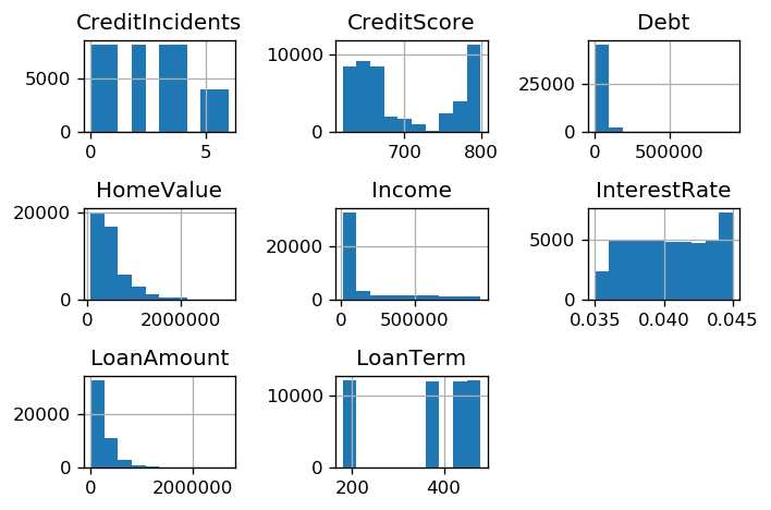

Customer Loans Dataset Histogram

df_customer[num_cols_customer].hist()
plt.tight_layout()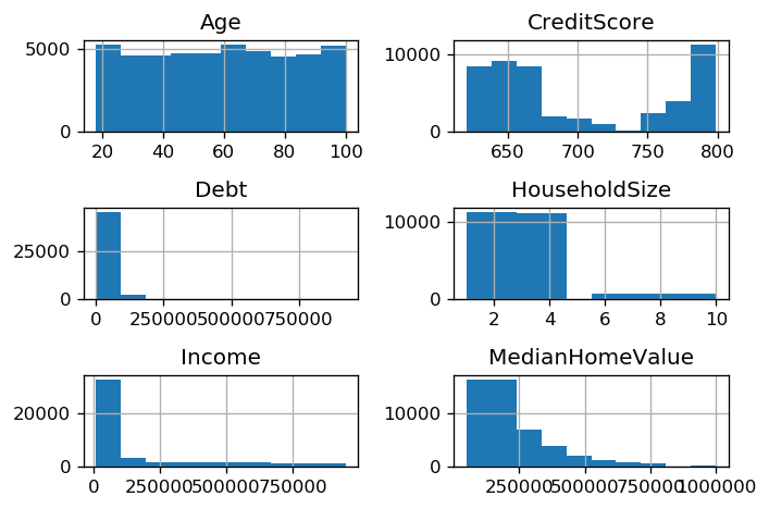

Demographics Dataset Histogram

Customer Location Heatmap

You generate a Heatmap that shows the location of the customers based on latitude ang longitude columns from the Demographics dataset. The red color on the Heatmap defines a higher density of customers.

latitudes = df_customer["Lat"]
longitudes = df_customer["Long"]

locations = np.array(list(zip(latitudes,longitudes)))
fig = gmaps.figure()
fig.add_layer(gmaps.heatmap_layer(locations))
fig

Join Datasets Together

You analyzed the datasets independently until now. Using the following code lines, you join the Customer Loans and Demographics datasets together. See the top 5 entries from the joined dataset.

cols_to_use = df_customer.columns.difference(df_loans.columns).tolist()
cols_to_use.append('custid')
df = df_loans.merge(df_customer[cols_to_use], on = 'custid')
df.head()

Create Features

This section demonstrates how to create a base feature set for your deep learning model. You use some of the columns from the previously joined data.

You build a neural network classifier which predicts “Approved” or “Denied” based on the input features.
The target variable is the column LoanStatus, which receives the values “Approved” or “Denied”.

num_features = ['Income','CreditScore','Debt','LoanTerm','InterestRate','CreditIncidents','HomeValue','LoanAmount',
               'HouseholdSize','Lat','Long','MedianHomeValue','MedianHouseholdIncome']
df_features = df[num_features]
df_product_type = pd.get_dummies(df.ProductType,prefix='ProductType')
df_features = pd.concat([df_features,df_product_type],axis=1)
features = df_features.values
targets = np.argmax(pd.get_dummies(df.LoanStatus).values,axis=1)

Scale Data

Scale your data using MinMaxScaler from sklearn library.

scaler=MinMaxScaler()
X = scaler.fit_transform(features)

Neural Network Model Creation

Start building your neural network model by defining two functions.

create_model - builds a feed forward neural network for binary classification

def create_model(input_shape):
    model = Sequential()
    model.add(Dense(128, input_dim=input_shape, activation='relu'))
    model.add(Dense(64, activation='relu'))
    model.add(Dropout(0.2))
    model.add(Dense(32, activation='relu'))
    model.add(Dense(16, activation='relu'))
    model.add(Dense(8, activation='relu'))
    model.add(Dense(1, activation='sigmoid'))
    model.compile(loss='binary_crossentropy', optimizer='sgd', metrics=['accuracy'])
    return model

train_and_evaluate_model - trains the network and returns the validation accuracy for the K-Fold cross validation

def train_and_evaluate__model(model, data_train, labels_train, data_test, labels_test):
    history = model.fit(data_train,labels_train,validation_data=(data_test,labels_test),epochs=30,batch_size=128)
    val_acc = history.history['val_accuracy'][-1]
    return val_acc, history

If you run this model on a Mac OS Machine, replace
val_acc = history.history['val_accuracy'][-1] 
with
val_acc = history.history['val_acc'][-1] 

K-Fold Cross Validation

In this section you set the K-Fold Cross Validation, that trains and tests the model with every data point from the train and test set. You use 3 different splits for training the model. After the run, if the Estimated Accuracy is closer to 1, the better is the model.

scores = []
models = []
historys = []
num_splits = 3
kf = KFold(n_splits=num_splits)
kf.get_n_splits(X)
input_shape = X.shape[1]

fold = 0
for train_index, test_index in kf.split(X):
    print("Running fold {}".format(fold))
    X_train, X_test = X[train_index], X[test_index]
    y_train, y_test = targets[train_index], targets[test_index]
    model = create_model(input_shape)
    score, history = train_and_evaluate__model(model,X_train,y_train,X_test,y_test)
    scores.append(score)
    models.append(model)
    historys.append(history)
    fold += 1
    
print('\n\nEstimated Accuracy ' , (np.round(np.mean(scores),2)), '  %')

Model Creation After K-Fold Cross Validation

If K-Fold Cross Validation accuracy is high, you can use your model for prediction.
Retrain your model with more train and test data, to fit the final model.

X_train, X_test, y_train, y_test = train_test_split(X, targets, test_size=0.20, random_state=42)
model = create_model(input_shape)
history = model.fit(X_train, y_train, validation_data=(X_test,y_test),epochs=30,batch_size=128)

Model Performance

The code lines below plot the loss and the accuracy for the train and test set.

plt.plot(history.history['loss'])
plt.plot(history.history['val_loss'])
plt.title('model loss')
plt.ylabel('loss')
plt.xlabel('epoch')
plt.legend(['train', 'test'], loc='upper left')
plt.show();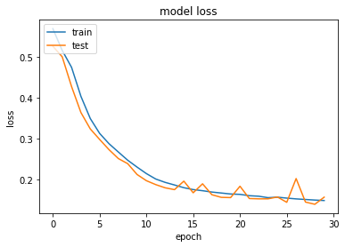

Model Performance - Loss

plt.plot(history.history['accuracy'])
plt.plot(history.history['val_accuracy'])
plt.title('model acc')
plt.ylabel('acc')
plt.xlabel('epoch')
plt.legend(['train', 'test'], loc='upper left')
plt.show();

If you run this model on a Mac OS Machine, replace:

plt.plot(history.history['accuracy'])

with

plt.plot(history.history['acc'])

and

plt.plot(history.history['val_accuracy'])

with

plt.plot(history.history['val_acc'])

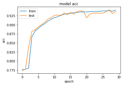
Model Performance - Accuracy

Final Code Review

Here are the code files discussed on this page.


#Data Handling and Manipulation
import pandas as pd
import numpy as np
pd.set_option('display.max_columns', None)  

#Statistical Analysis
from scipy import stats

#Plotting and Visualization
import matplotlib.pyplot as plt
import matplotlib.pylab as plt
plt.rcParams['figure.dpi'] = 120
import gmaps
!jupyter nbextension enable --py gmaps

#Machine Learning
from sklearn.preprocessing import MinMaxScaler
from keras.models import Sequential
from keras.layers import Dense, Dropout
from sklearn.model_selection import cross_val_score, train_test_split
from sklearn.model_selection import KFold
from sklearn.ensemble import RandomForestClassifier
df_loans = pd.read_csv('Data/customer_loans.csv',sep=',')
df_loans.head()
df_customer = pd.read_csv('Data/customer_demographics.csv',sep=',')
df_customer.head()
df_loans.isna().sum()
df_customer.isna().sum()

num_cols_loans = ['Income','CreditScore','Debt','LoanTerm','InterestRate','CreditIncidents','HomeValue','LoanAmount']
df_loans[(np.abs(stats.zscore(df_loans[num_cols_loans])) > 3).all(axis=1)]

num_cols_customer = ['Age','Income','CreditScore','HouseholdSize','MedianHomeValue','Debt']
df_customer[(np.abs(stats.zscore(df_customer[num_cols_customer])) > 3).all(axis=1)]

df_loans[num_cols_loans].describe()
df_customer[num_cols_customer].describe()

df_loans[num_cols_loans].hist()
plt.tight_layout()

df_customer[num_cols_customer].hist()
plt.tight_layout()

latitudes = df_customer["Lat"]
longitudes = df_customer["Long"]

locations = np.array(list(zip(latitudes,longitudes)))
fig = gmaps.figure()
fig.add_layer(gmaps.heatmap_layer(locations))
fig


cols_to_use = df_customer.columns.difference(df_loans.columns).tolist()
cols_to_use.append('custid')
df = df_loans.merge(df_customer[cols_to_use], on = 'custid')
df.head()

num_features = ['Income','CreditScore','Debt','LoanTerm','InterestRate','CreditIncidents','HomeValue','LoanAmount',
               'HouseholdSize','Lat','Long','MedianHomeValue','MedianHouseholdIncome']
df_features = df[num_features]
df_product_type = pd.get_dummies(df.ProductType,prefix='ProductType')
df_features = pd.concat([df_features,df_product_type],axis=1)
features = df_features.values
targets = np.argmax(pd.get_dummies(df.LoanStatus).values,axis=1)

scaler=MinMaxScaler()
X = scaler.fit_transform(features)

def create_model(input_shape):
    model = Sequential()
    model.add(Dense(128, input_dim=input_shape, activation='relu'))
    model.add(Dense(64, activation='relu'))
    model.add(Dropout(0.2))
    model.add(Dense(32, activation='relu'))
    model.add(Dense(16, activation='relu'))
    model.add(Dense(8, activation='relu'))
    model.add(Dense(1, activation='sigmoid'))
    model.compile(loss='binary_crossentropy', optimizer='sgd', metrics=['accuracy'])
    return model
    
    def train_and_evaluate__model(model, data_train, labels_train, data_test, labels_test):
    history = model.fit(data_train,labels_train,validation_data=(data_test,labels_test),epochs=30,batch_size=128)
    val_acc = history.history['val_accuracy'][-1]
    return val_acc, history
    
    scores = []
models = []
historys = []
num_splits = 3
kf = KFold(n_splits=num_splits)
kf.get_n_splits(X)
input_shape = X.shape[1]

fold = 0
for train_index, test_index in kf.split(X):
    print("Running fold {}".format(fold))
    X_train, X_test = X[train_index], X[test_index]
    y_train, y_test = targets[train_index], targets[test_index]
    model = create_model(input_shape)
    score, history = train_and_evaluate__model(model,X_train,y_train,X_test,y_test)
    scores.append(score)
    models.append(model)
    historys.append(history)
    fold += 1
    
print('\n\nEstimated Accuracy ' , (np.round(np.mean(scores),2)), '  %')

X_train, X_test, y_train, y_test = train_test_split(X, targets, test_size=0.20, random_state=42)
model = create_model(input_shape)
history = model.fit(X_train, y_train, validation_data=(X_test,y_test),epochs=30,batch_size=128)

plt.plot(history.history['loss'])
plt.plot(history.history['val_loss'])
plt.title('model loss')
plt.ylabel('loss')
plt.xlabel('epoch')
plt.legend(['train', 'test'], loc='upper left')
plt.show();

plt.plot(history.history['accuracy'])
plt.plot(history.history['val_accuracy'])
plt.title('model acc')
plt.ylabel('acc')
plt.xlabel('epoch')
plt.legend(['train', 'test'], loc='upper left')
plt.show();